The National Energy Market in Australia uses a standard format for exchanging meter data. For interval meter read from smart meters this standard is called NEM12.
NEM12 files contain details about energy consumed and exported to the grid in 30, 15 or 5 minute intervals. This data is used by retailers to bill customers and by distributors to plan network upgrades.
This data is also pretty handy for consumers to understand energy efficiency and also double check their electricity bills.
Some distributors like United Energy allow download of this data for home meters via their My Energy portal.
Challenge
NEM12 meter data files are semi-structured. This can present issues when exporting data into a spreadsheet tool or loading into a database.
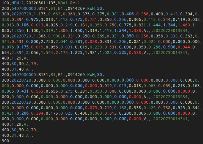
Example input data:
Whilst the file is comma separated, each line consists of a distinct record type according to the file format specification.
Additionally, valid files are defined by a block cycle defined in the file specification. For example, context about 300 records is determined by the preceding 200 block. This means details relevant for analysis are often present on multiple lines of the file, even when looking at a single day’s worth of meter reads.
Additional complexity:
Multiple meters might exist in a single file
Mixed interval granularities
Mixed units of measure / scales
Read quality is stored separately to numeric values (this can occur when some reads on a day are estimates e.g. due to meter communication issues)
Solution
The solution is a custom NEM12 reader Node module which parses NEM12 and converts to more convenient human / machine readable output formats.
The module provides a convenient way to transform the semi-structured NEM12 file format into something more useful for ad-hoc analysis or ingestion into a data platform.
The module could also be integrated into front-end or back-end analytics applications.
Future improvements could include stricter validation of input files (e.g. where data types should only contain certain values) and additional output formats (e.g. a 5 minute output which disaggregates less granular meter data).
AEMO is the Australian Energy Market Operator. It makes available a well organised database for market participants to track bids, demand, generation and other market functions. This database is known as the MMS (Market Management System Data Model).
Electricity researchers, retailers, distributors and others use this data to get insights and manage their business.
The traditional approach to make use of MMS datasets is to load them into an RDBMS. The volume, and variety of data can make this difficult, although some helper tools do exist. However loading a large history of granular data for analysis, even for a particular dataset is also a common business requirement.
Apache Spark (an alternative to traditional RDBMS) has a natural advantage in being able to read and process large datasets in parallel, particularly for analytics.
Can it be used here?
Challenges
The AEMO CSV format used to populate MMS allows there to be multiple reports in a single file.
Furthermore files are frequently compressed in Zip format. This usually means pre-processing is required – e.g. before reading in as text or CSV.
Whilst the underlying files are comma separated, the number of columns in each row also varies in a given file due to:
Different record types (Comment, Information or Data)
Different report schemas (each having a different column set)
AEMO MMS Data Model CSV structure
Here is a snippet from a sample file:
C,SETP.WORLD,DVD_DISPATCH_UNIT_SCADA,AEMO,PUBLIC,2021/10/07,00:00:05,0000000350353790,,0000000350353744
I,DISPATCH,UNIT_SCADA,1,SETTLEMENTDATE,DUID,SCADAVALUE
D,DISPATCH,UNIT_SCADA,1,"2021/09/01 00:05:00",BARCSF1,0
D,DISPATCH,UNIT_SCADA,1,"2021/09/01 00:05:00",BUTLERSG,9.499998
D,DISPATCH,UNIT_SCADA,1,"2021/09/01 00:05:00",CAPTL_WF,47.048004
...lots more rows...
C,"END OF REPORT",3368947
This file structure presents some specific challenges for parsing with Spark and thus being able to derive useful insights from the underlying data.
Issue #1 – reading too many rows in a file (even for a single report) can cause out of memory issues
Issue #2 – naively reading just the data (D) rows misses file and report header information, such as column names
Issue #3 – parsing full files can result in unnecessary data being read, when only a subset is needed
Solution
SparkMMS is a custom data reader implemented in Java using Apache Spark’s DataSource V2 API.
It can be used to efficiently read AEMO MMS files in bulk.
Input:
SparkMMS takes a glob path, which means it can read multiple files based on a file pattern – e.g. to read all dispatch related zip files from a monthly archive:
Spark MMS creates a Spark dataframe with chunks of rows related to each specific report type across all input files. The data rows are nested in the “data” column of the dataframe. The file header, report headers (including column names) and data rows are also preserved:
This structure makes it easy to do further processing of the data and means no information is lost when reading files in parallel:
Other features:
Reads both .CSV and .zip
Automatically splits large files into multiple partitions
Extracts useful metadata from raw files, including column headers
Supports multiple report schemas / versions
Supports predicate pushdown – skips reports within a file if not selected
Column pruning – reads of only a subset of data from raw files, if columns not selected
Can read from cloud storage (e.g. Azure Blob storage, Amazon S3, Databricks DBFS)
Demo
These steps show the SparkMMS custom reader in action using Azure Databricks:
Note: Databricks is a paid cloud based Data Lake / ML platform. Alternatively, see source code for a demonstration running Spark MMS locally on a single node.
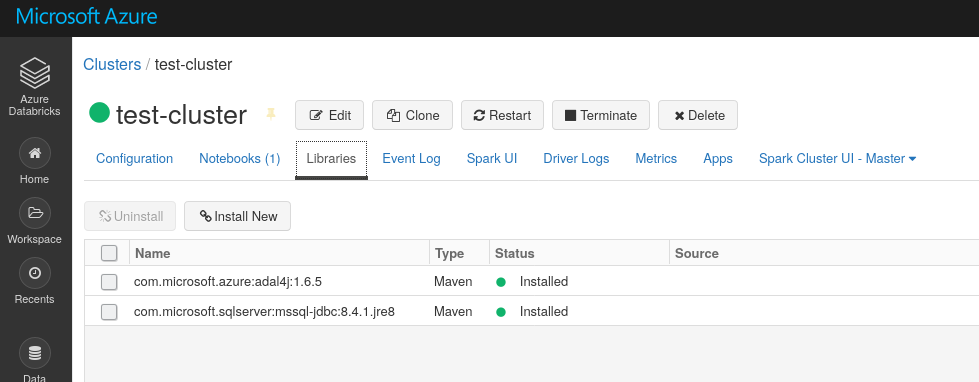
Start a Databricks cluster – e.g.: Note: Select Runtime 9.1 LTS for compatibility
Add the SparkMMS library to the cluster via Cluster > Libraries > Install New > Drag and Drop Jar:
Using SparkMMS
1. Define helper functions. At runtime, these create MMS report specific dataframe definitions (with correct per-report column headings) and also create temporary tables to streamline querying via SQL:
# Get a new dataframe with the schema of a single report type
def getReport(df, report_type, report_subtype, report_version):
    from pyspark.sql.functions import explode
    df = df.where(f"report_type = '{report_type}' and report_subtype = '{report_subtype}' and report_version = {report_version}")
    tmpDF = df.select("column_headers", explode(df.data).alias("datarow"))

    colHeaders = df.select("column_headers").first().column_headers

    for idx, colName in enumerate(colHeaders):
        tmpDF = tmpDF.withColumn(colName, tmpDF.datarow[idx])

    tmpDF = tmpDF.drop("column_headers").drop("datarow")

    return tmpDF

# Register all reports available in the dataframe as temporary view in the metastore
def registerAllReports(df=df):
    tmpDF = df.select("report_type","report_subtype","report_version")
    tmpDF = tmpDF.dropDuplicates()

    reports = tmpDF.collect()

    for r in reports:
        tmpReportDF = getReport(df,r.report_type,r.report_subtype,r.report_version)
        tmpReportDF.createOrReplaceTempView(f"{r.report_type}_{r.report_subtype}_{r.report_version}")
2. Create a temporary directory and download sample data from AEMO (15mb zipped, 191mb unzipped):
%sh
cd /dbfs/
mkdir tmp
cd tmp
wget https://nemweb.com.au/Data_Archive/Wholesale_Electricity/MMSDM/2021/MMSDM_2021_09/MMSDM_Historical_Data_SQLLoader/DATA/PUBLIC_DVD_DISPATCH_UNIT_SCADA_202109010000.zip
Note – there is no need to unzip the file.
3. Read raw data into a Spark dataframe using SparkMMS:
Notes:
Option maxRowsPerPartition tells the reader to create each partition with a maximum of 50,000 report data rows. All report rows will be read, however some will be in different partitions for performance reasons.
Option minSplitFilesize tells the reader not to bother splitting files smaller than 1,000,000 bytes, which improves performance.
Note: Optionally here we can also run df.cache() to improve performance in subsequent steps.
5. Register each report found in the raw file(s) as a temporary table and then validate the output:
registerAllReports(df)
After the above command, a single temp table is registered because our file only contained one report: Report type: DISPATCH Report sub-type: UNIT_SCADA Version: 1
Note: If we selected more files in step 2 above we would see more temp tables above.
Now query the temp table and check the data:
6. Finally, we can create a view on top of the temporary table(s) with further calculations or data-type conversions – for example:
%sql
-- Create a temporary view with expected data types
CREATE OR REPLACE TEMPORARY VIEW vw_dispatch_unit_scada_1
AS
SELECT
  to_timestamp(REPLACE(SETTLEMENTDATE,'"',''), 'yyyy/MM/dd HH:mm:ss') AS dispatch_time, -- Strip quote characters from SETTLEMENTDATE and convert to native timestamp type
  DUID AS generator,
  CAST(SCADAVALUE AS DOUBLE) AS generation_MW -- Convert to numeric
FROM dispatch_unit_scada_1;
…and then perform charting, aggregations. For example, charting the average generation in MW for three generation units (Coal, Wind, Solar) in September 2021:
Conclusion
Apache Spark provides a convenient way to process large datasets in parallel once data is available in a structured format.
AEMO’s MMS data model data is vast and varied, so keeping all data loaded in an online platform for eternity can be an expensive option. Occasionally, however, a use case may arise which relies on having a long period of historical data available to query.
SparkMMS demonstrates a convenient way to process raw files in bulk, with no pre-processing or manual schema design. In some organisations, historical files may be available on cloud / local storage, even if data has been archived from an RDBMS. Therefore, custom readers like SparkMMS may be a convenient option to explore for ad-hoc use cases, as an alternative to re-loading old data into a relational database.
Sometimes it’s handy to be able to test Apache Spark developments locally. This might include testing cloud storage such as WASB (Windows Azure Storage Blob).
These steps describe the process for testing WASB locally without the need for an Azure account. These steps make use of the Azurite Storage Emulator.
Steps
Prerequisites
Download and extract Apache Spark (spark-3.1.2-bin-hadoop3.2.tgz)
Create a new directory and start the Azurite Storage Emulator Docker container – e.g.:
mkdir ~/blob
docker run -p 10000:10000 -p 10001:10001 -v /home/david/blob/:/data mcr.microsoft.com/azure-storage/azurite
NB – in the above example, data will be persisted to the local linux directory /home/david/blob.
Upload files with Storage Explorer:
Connect Storage Explorer to the Local Storage emulator (keep defaults when adding the connection):
Upload a sample file – e.g. to the “data” container:
Start Spark using the packages option to include libraries needed to access Blob storage. The Maven coordinates are shown here are for the latest hadoop-azure package:
cd ~/spark/spark-3.1.2-bin-hadoop3.2/bin ./pyspark --packages org.apache.hadoop:hadoop-azure:3.3.1
The PySpark shell should start as per normal after downloading hadoop-azure and its dependencies.
Troubleshooting: The following stack trace indicates the hadoop-azure driver or dependencies were not loaded successfully: ... py4j.protocol.Py4JJavaError: An error occurred while calling o33.load. : java.lang.RuntimeException: java.lang.ClassNotFoundException: Class org.apache.hadoop.fs.azure.NativeAzureFileSystem not found at org.apache.hadoop.conf.Configuration.getClass(Configuration.java:2595) at org.apache.hadoop.fs.FileSystem.getFileSystemClass(FileSystem.java:3269) ... Caused by: java.lang.ClassNotFoundException: Class org.apache.hadoop.fs.azure.NativeAzureFileSystem not found at org.apache.hadoop.conf.Configuration.getClassByName(Configuration.java:2499) at org.apache.hadoop.conf.Configuration.getClass(Configuration.java:2593) ... 25 more ...
Ensure the “packages” option is correctly set when invoking pyspark above.
Query the data using the emulated Blob storage location from the PySpark shell:
Notes: data – container where the data was uploaded earlier @storageemulator – this is a fixed string used to tell the WASB connector to point to the local emulator
Example output:
Conclusion
Local storage emulation allows testing of wasb locations without the need to connect to a remote Azure subscription / storage account.
The Delta Lake format in Databricks provides a helpful way to restore table data using “time-travel” in case a DML statement removed or overwrote some data.
The goal of a restore is to bring back table data to a consistent version.
Delta lake timetravel
This allows accidental table operations to be reverted.
Example
Original table – contains 7 distinct diamond colour types including color = “G”:
Original table
Then, an accidental deletion occurs:
Accidental SQL delete statement
The table is now missing some data:
Modified table
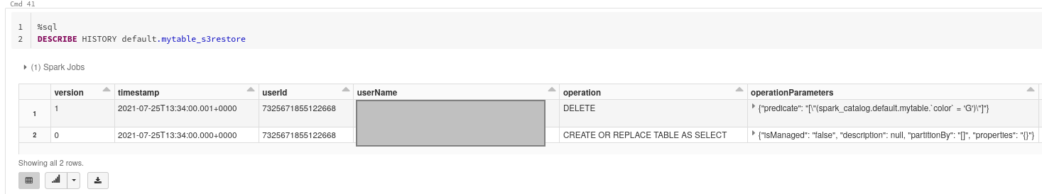
However, we can bring back the deleted data by checking the Delta Lake history and restoring to a version or timestamp prior to when the delete occurred – in this case version 0 of mytable:
Delta Lake table history
Restoring the original table based on a timestamp (after version 0, but prior to version 1):
%sql
DROP TABLE IF EXISTS mytable_deltarestore;

CREATE TABLE mytable_deltarestore
USING DELTA
LOCATION "s3a://<mybucket>/mytable_deltarestore"
AS SELECT * FROM default.mytable TIMESTAMP AS OF "2021-07-25 12:20:00";
Now, the original data is available in the restored table, thanks to Delta Lake time-travel:
Restored data – via Timetravel
Challenge
What happens if table files (parquet data files or transaction log files) have been deleted in the underlying storage?
This might occur if a user or administrator accidentally deletes objects from S3 cloud storage.
Two types of files might get deleted manually.
Delta Lake data files
Symptom – table is missing data and can’t be queried:
%sql
SELECT * FROM mytable@v0;

(1) Spark Jobs
FileReadException: Error while reading file s3a://<mybucket>/mytable/part-00000-1932f078-53a0-4cbe-ac92-1b7c48f4900e-c000.snappy.parquet. A file referenced in the transaction log cannot be found. This occurs when data has been manually deleted from the file system rather than using the table `DELETE` statement. For more information, see https://docs.microsoft.com/azure/databricks/delta/delta-intro#frequently-asked-questions
Caused by: FileNotFoundException: No such file or directory: s3a://<mybucket>/mytable/part-00000-1932f078-53a0-4cbe-ac92-1b7c48f4900e-c000.snappy.parquet
Delta Lake transaction logs
Symptom – table state is inconsistent and can’t be queried:
%sql
FSCK REPAIR TABLE mytable DRY RUN

Error in SQL statement: FileNotFoundException: s3a://<mybucket>/mytable/_delta_log/00000000000000000000.json: Unable to reconstruct state at version 1 as the transaction log has been truncated due to manual deletion or the log retention policy (delta.logRetentionDuration=30 days) and checkpoint retention policy (delta.checkpointRetentionDuration=2 days)
Solution
Versioning can be enabled for S3 buckets via the AWS management console:
This means that if any current object versions are deleted after the above configuration is set, it may be possible to restore them.
Databricks Delta Lake tables are stored on S3 under a given folder / prefix – e.g.:
s3a://<mybucket>/<mytable>
If this prefix can be restored to a “point in time”, this can be used to restore a non-corrupted version of a table – for example:
NB: Restoring will mean all data added after deletion occurs will be lost and would need to be reloaded from an upstream source. This also assumes that previous object versions are available on S3.
The following steps can be used in Databricks to restore past S3 object versions to a new location and re-read the table at the restore point:
Install the s3-pit-restore python library in a new Databricks notebook cell: %pip install s3-pit-restore
Run the restore command with a timestamp prior to the deletion: %sh export AWS_ACCESS_KEY_ID="<access_key_id>" export AWS_SECRET_ACCESS_KEY="<secret_access_key>" export AWS_DEFAULT_REGION="<aws_region>" s3-pit-restore -b <mybucket> -B <mybucket> -p mytable/ -P mytable_s3restore -t "25-07-2021 23:26:00 +10"
Create a new table pointing to the restore location: %sql CREATE TABLE mytable_s3restore USING DELTA LOCATION "s3a://<mybucket>/mytable_s3restore/mytable";
Verify the table contents are again available and no longer corrupted:
Conclusion
Other techniques like Table Access Control may be preferable to prevent Databricks users from deleting underlying S3 data, however Point in Time restore techniques may be possible where table corruption has occurred and S3 bucket versioning is enabled.
Solar PV inverters often have their own web-based monitoring solutions. However some of these do not make it easy to view current generation or consumption due to refresh delays. Out of the box monitoring is usually good for looking at long-term time periods however lacks the granularity to see consumption of appliances over the short term.
The challenge
Realtime monitoring of Solar generation and net export helps to maximise self-consumption. For example coordinating appliances to make best use of solar PV.
Existing inverter monitoring does not show granular data over recent history – for example, to be able to tell when a dishwasher has finished its heating cycle and whether another high-consumption appliance should be turned on:
Solution
This sample android application allows realtime monitoring whilst charting consumption, generation and net export:
The chart shows recent data over time and is configurable for SMA and Enphase inverters. In both cases the local interface of each inverter is used to pull raw data:
Improve security handling of SSL – the current code imports a self-signed SMA inverter certificate and disables hostname verification to allow the SMA local data to be retrieved
Refine code and publish to an app store
Remove hard-coding for extraction of metrics
Better error handling
Add a data export function
Conclusion
This sample app is really handy to monitor appliances in realtime and allows making informed decisions about when to start appliances.
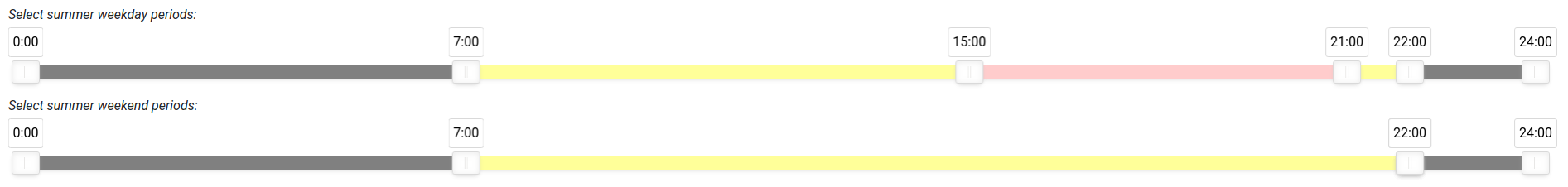
Electricity retailers sometimes give the choice of paying a flat rate for electricity, or so called Time of Use (ToU) rate. Time of use pricing usually has peak, off-peak and shoulder prices. This can also vary by time of year and also weekend or weekday.
For the consumer, Time of Use pricing may be beneficial if consumption can be shifted to off-peak hours, but this is potentially offset by more expensive rates during peak times.
Assuming a retailer gives the ability to choose – which one is cheaper?
Solution
This web calculator gives the ability to simulate costs based on historical meter data usage and configurable pricing and peak/off-peak definition:
Note: Beta only. Default prices may be different depending on the retailer or electricity plan, but the sliders allow adjustment to configure unit prices to match any real plan for comparison.
Features
Calculate costs, potential savings and get a recommendation:
Fully client-side, JavaScript and HTML – no server upload required
Ability to drag-and-drop upload a Victorian Energy Compare formatted CSV:
Focus on a particular date range within the uploaded meter data:
Ability to configure time of use definitions (i.e. peak, off-peak and shoulder times):
Potential future improvements
The following future improvements could make the solution more useful:
Cope with different data formats (different States’ data)
Ability to compare two (or n) different plans
Automatic comparison of available plans from multiple retailers (pulling prices automatically)
Inclusion of solar feed-in tariff as a comparison point
Provide recommendations for changing energy usage behaviour
The code is experimental and proof of concept only – it has not been fully tested
The code runs as a Linux service
It features a web UI
It checks home energy consumption and decides whether to turn the plug on or off based on a threshold
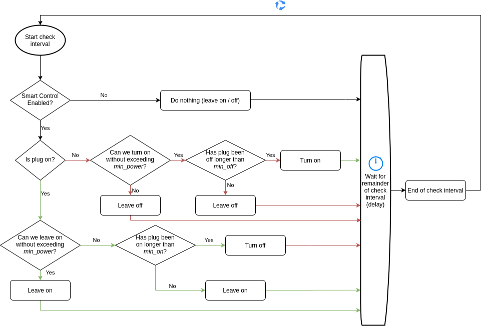
The logic
For each check interval the code checks the current state of the plug and decides whether to:
Do nothing
Leave on
Leave off
Turn on
Turn off
Here’s a flowchart showing the decision-making process:
The Web UI
The features
Ability to disable / enable automatic control
This is useful where the plug needs to be manually controlled via its physical button
Configurable Min power threshold
This is useful where it’s acceptable to use some grid power as well as solar (e.g. partly cloudy weekends with cheaper electricity rates)
Minimum on / off buffer periods to reduce switching (e.g. for devices which do not benefit from being powered on and off continually)
Monitoring messages to see how many times the switch has been controlled and its last state
Overall net ( W )
Useful for seeing current net household energy consumption
Automatic recovery if the plug, solar monitoring API or Wifi network goes offline temporarily
The result
So far this solution works great.
On a partially cloudy day, the plug automatically turns on or off once excess solar drops below the min power threshold. Similarly, the plug will turn off when household consumption is high – for example, during the heating cycle of a washing machine / dishwasher or when an electric kettle is used.
We got an interesting email from our electricity retailer after setting up this solution:
Email from our electricity retailer
The message indicates we have successfully boosted our self-consumption – i.e. more solar energy is being self-consumed rather than being exported to the grid, giving the appearance to the retailer that the solar PV system is underperforming. Success!
Conclusion
This is not quite as good as having a home battery or a dedicated (and much more refined) device like the Zappi, however it comes close. It is a great way to boost self-consumption of excess solar PV energy using software and a low-cost smart plug. With around a year of weekly charging, this solution can pay for the cost of the smart plug by reducing the effective cost of electricity.
This is pretty amazing for EV owners who also have solar PV.
It means that instead of exporting surplus energy at a reduced rate ($0.12/kWh) it is possible to avoid importing energy at a higher rate ($0.25/kWh). This can effectively double the benefit of having solar PV by boosting self consumption.
However as of writing, the Zappi V2 is $1,395 (for example, from EVolution here).
Challenge
Is it possible to create a software virtual plug to charge an EV using only self-generated solar PV?
The idea
Charging the EV using only rooftop solar costs $0.12/kWh. This is the opportunity cost of the feed-in tariff which would would otherwise be earned for feeding energy into the grid.
Charging the EV using grid power alone costs around $0.25/kWh.
Depending on the proportion of PV generation at a given time, the effective cost per kWh may be somewhere in between.
What if we can turn on the charger only at times when the solar is generating 100% or more of what the EV will use?
A custom software program could query net solar export and control a smart plug to generate savings.
Equipment
Mitsubishi Outlander PHEV
Envoy S Metered Solar house monitor
TP Link HS110 Smart Plug
Potential benefits
Cheaper EV charging (approximately 50% savings)
No need to manually enable / disable charging when:
Weather is variable
Household consumption is high (e.g. boiling a kettle or running the dishwasher)
Things to consider
These are also some risks to consider when designing a DIY software control:
The PHEV plug safety instructions say not to plug anything in between the wall socket and charger plug – i.e. where the SmartPlug should go.
The PHEV charger expects to be plugged in and left alone – will it be happy with power being enabled / disabled?
Another thing to consider… is it worth buying a Smartplug to do this?
Assuming the plug can be purchased for a reasonable price (for example $40 including shipping from here) and weekly EV charging from nearly empty, the plug pays itself off in <1 year:
Plug cost:
40.00
Opportunity cost / lost export ($/kWh):
0.12
Saved expense ($/kWh):
0.25
Net saving ($/kWh):
0.13
kWh savings to pay off:
307.69
Average charging session (kWh):
8.00
Number of charges:
38.46
Back of the envelope calculations
Continued…
See Part 2 for an approach to implement this solution in Python…
When using Databricks 5.5 LTS to read a table from SQL Server using Azure Active Directory (AAD) authentication, the following exception occurs:
Error : java.lang.NoClassDefFoundError: com/microsoft/aad/adal4j/AuthenticationException Error : java.lang.NoClassDefFoundError: com/microsoft/aad/adal4j/AuthenticationException
 at com.microsoft.sqlserver.jdbc.SQLServerConnection.getFedAuthToken(SQLServerConnection.java:3609)
 at com.microsoft.sqlserver.jdbc.SQLServerConnection.onFedAuthInfo(SQLServerConnection.java:3580)
 at com.microsoft.sqlserver.jdbc.SQLServerConnection.processFedAuthInfo(SQLServerConnection.java:3548)
 at com.microsoft.sqlserver.jdbc.TDSTokenHandler.onFedAuthInfo(tdsparser.java:261)
 at com.microsoft.sqlserver.jdbc.TDSParser.parse(tdsparser.java:103)
 at com.microsoft.sqlserver.jdbc.SQLServerConnection.sendLogon(SQLServerConnection.java:4290)
 at com.microsoft.sqlserver.jdbc.SQLServerConnection.logon(SQLServerConnection.java:3157)
 at com.microsoft.sqlserver.jdbc.SQLServerConnection.access$100(SQLServerConnection.java:82)
 at com.microsoft.sqlserver.jdbc.SQLServerConnection$LogonCommand.doExecute(SQLServerConnection.java:3121)
 at com.microsoft.sqlserver.jdbc.TDSCommand.execute(IOBuffer.java:7151)
 at ...io.netty.util.concurrent.DefaultThreadFactory$DefaultRunnableDecorator.run(DefaultThreadFactory.java:138)
 at java.lang.Thread.run(Thread.java:748) Caused by: java.lang.ClassNotFoundException: com.microsoft.aad.adal4j.AuthenticationException
 at java.net.URLClassLoader.findClass(URLClassLoader.java:382)
 at java.lang.ClassLoader.loadClass(ClassLoader.java:418)
 at sun.misc.Launcher$AppClassLoader.loadClass(Launcher.java:352)
 at java.lang.ClassLoader.loadClass(ClassLoader.java:351) ... 59 more...
1 – Create a new init script which will remove legacy MSSQL drivers from the cluster. The following commands create a new directory on DBFS and then create a shell script with a single command to remove mssql driver JARs:
It’s easy in the digital age to amass tens of thousands of photos (or more!). Categorising these can be a challenging task, let alone searching through them to find that one happy snap from 10 years ago.
Significant advances in machine learning over the past decade have made it possible to automatically tag and categorise photos without user input (assuming a machine learning model has been pre-trained). Many social media and photo sharing platforms make this functionality available for their users — for example, Flickr’s “Magic View”. What if a user has a large number of files stored locally on a Hard Disk?
The problem
49,049 uncategorised digital images stored locally
Manual categorisation
No easy way to search (e.g. “red dress”, “mountain”, “cat on a mat”)